Millions of people around the world use Microsoft Excel to handle all kinds of office and productivity tasks. It's an easy program to pick up and most people become comfortable using it very quickly.
But to truly master it, you can either spend years working your way through endless tasks, or you can join us as we take a quick look at some of the top 10 shortcuts, tips, and hacks that will help you on your way to becoming an Excel pro in no time at all.
1. (Short)cut to the chase
Like most other programs, Excel has keyboard shortcuts programmed into it, so you don't have to click all over the screen, or work your way through numerous menus to get something done.
The only problem is there are a LOT of shortcuts – far too many to list them all here. However, the more recent versions of Excel will show you all the keys to press to access options from the ribbon.
Just press ALT to show which key you need for a tab on the ribbon (e.g. the Insert menu is N), and then you'll see the key(s) for each option. Alternatively, resting the cursor over the option you want will show a tooltip, displaying the corresponding keyboard shortcut, too.
For example, the shortcut for 3D Shapes is ALT, then N, followed by S, and finally 3. Don't press them all together – do each key successively. If you want to see keyboard shortcuts for specific tasks, Microsoft has a nice list for all versions of Excel.
The idea is that for certain repetitive tasks, you can develop some muscle memory and get going just as you do copying and pasting. They're so useful for speeding up productivity that you'll find a few more of them throughout this article.
2. Double-click to fill in quick
If you have large sets of data that you need to run the same formula for, you don't need to drag or copy the original formula cell across all the others.
Simply place the mouse cursor over the bottom right corner of the cell – the cursor will change shape and color.
That's when you can double-click and the formula will be copied down for as many cells as there is adjacent data.
The same can be accomplished using the keyboard (faster): use CTRL + D to fill a single or multiple cell selection.
3. Making charts and graphs the professional way
Presenting data in the form of charts or graphs is another staple task of most Excel users. There's a wealth of types and formatting options to choose from, though, so it's not always easy to know what's best to use or how to go about doing something.
Here are a few tips to keep your data visualizations looking clean and crisp.
First of all, make sure you match the right chart type to the data you have – for example, data from categorical variables (e.g. revenue per quarter, number of sales of a given item) should be displayed using a bar or pie chart, or a line graph.
Data from sets of continuous variables (e.g. reaction rates vs. concentration) should be displayed using XY scatter graphs.
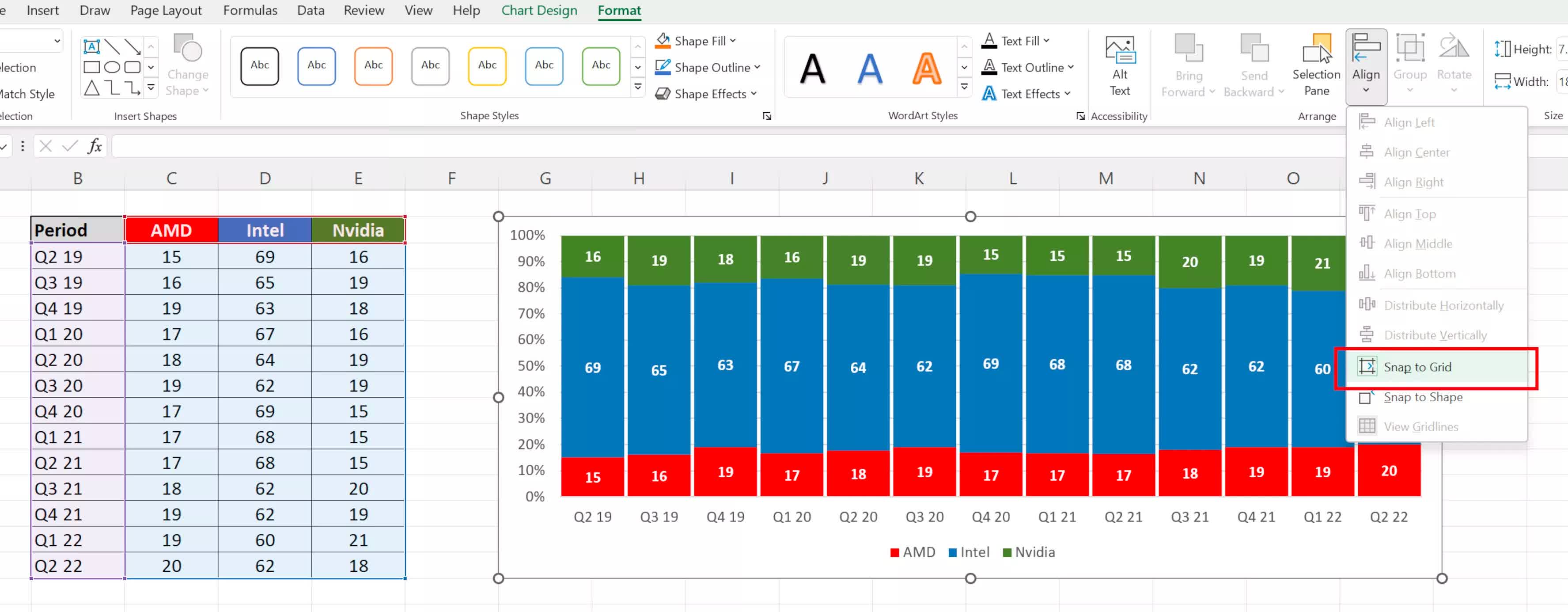
Graphs embedded in worksheets can be aligned with cell boundaries either by holding down ALT when you move it about or by enabling Snap to Grid in the graph's format options (click on the graph, then press ALT, J, A, A, A, P).
Also, don't feel that you need to add a legend to every chart you make: in pie charts, there's often plenty of room to add that information into the slices themselves, but rarely so in the case of bar charts.
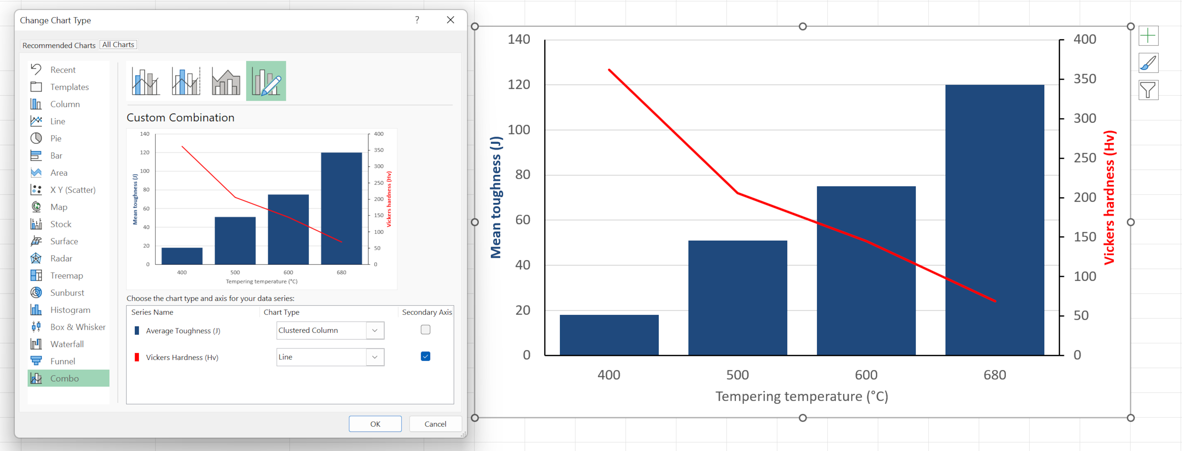
If you want to display two different chart types in the same one, you can do this by highlighting the data you want to show on the same chart, then selecting Combo from the chart selection window (ALT, N, K).
Note that when making a combo graph, it's a good idea to put one of the data series on a secondary axis – this means you can have two different vertical scales showing, boosting the value of the chart.
4. One key mastery
When copying formulae across cells, sometimes you want it to always use one fixed value against all the others. To lock a cell, row, or column in a formula, you need to apply a dollar sign before the letter or number.
So let's say the formula is =C3*D3 and we want to stick and always use the value in cell C3.
The formula will now read as =$C$3*D3 and will always use C3, no matter where you copy the formula to.
A quick way to apply those dollar signs when typing your formula is to hit F4 in your keyboard, and bingo! It works just as well with highlighting a single character, such as a column label, and then pressing F4.
The F4 function key can also be used in Excel to repeat the last action, for example, if you shaded a cell in a particular color and want to repeat the same action to another cell, just hit F4.
5. Type once, fill many
If you need to enter the same data into multiple cells, no matter where they are, there's a quick way to do this. Select the row, column, or cells you want to add the same value into.
Note, if the cells are scattered about the spreadsheet, hold CTRL down while you left-click the cells you want.

While the selected cells are still all highlighted, type the value you want to enter (text and/or numbers), then press CTRL + Enter. You'll now have a raft of new cells all nicely filled in!
6. Fast tables, fast graphs, fast analysis
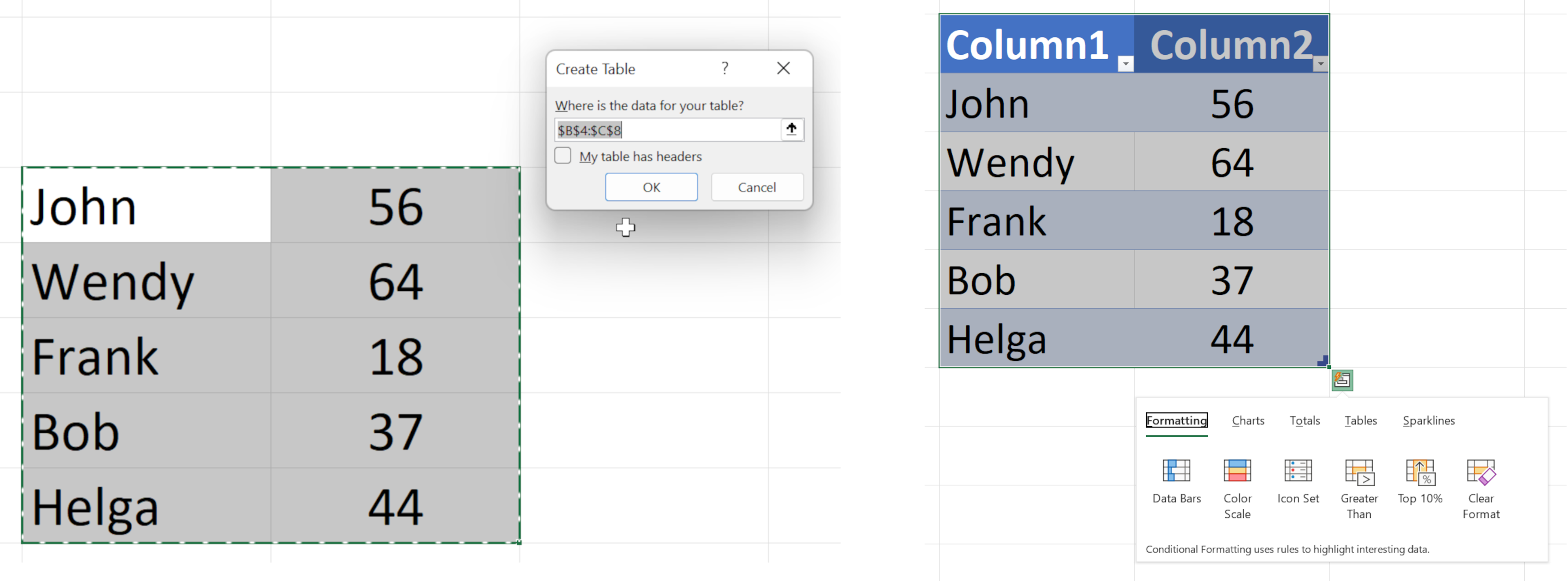
Tables are a great way of presenting data for easier reading and yes, there's a fast way of churning them out. Highlight the cells you want in the table, press ALT, followed by N, then T.
You'll see a window confirming the selection you've chosen, so after this, you just press Enter. You'll see there are automatic filters for each column and a tag in the bottom right-hand corner that, clicked and held onto, always you to drag out extra rows or columns.
With your table finished, right-click on any part of it, and select the Quick Analysis option in the middle. Here, you can quickly alter the format of the table, add in some automatic calculations and conditional formatting, charts, and a pivot table.
And speaking of pivot tables...
7. Tackling tremendous tables without trepidation
Regular Excel users may face having to juggle large tables of data all the time. Hacking your way through them, to compare different aspects, can be tiresome and lead to errors when trying to read the information.
Pivot tables allow you to filter data based on just the sections you want, making it easier to analyze and summarize information from a large data set. Pivot tables never affect the data source, so you can chop and change pivot tables without worrying about deleting something important.
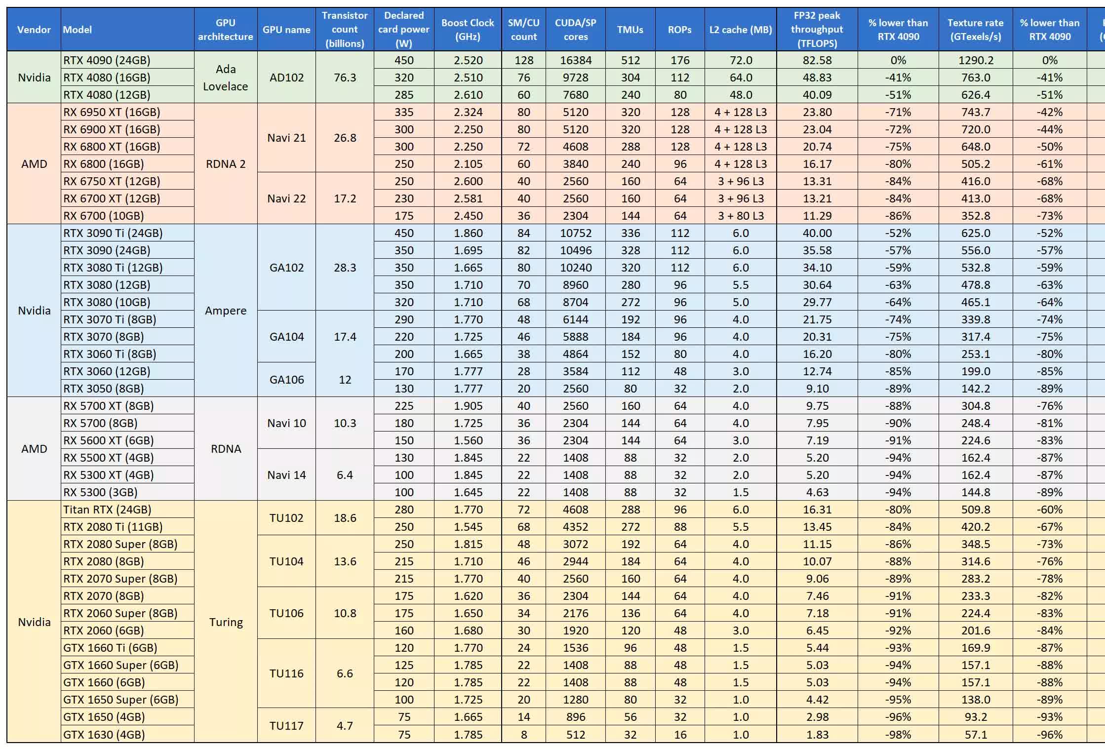
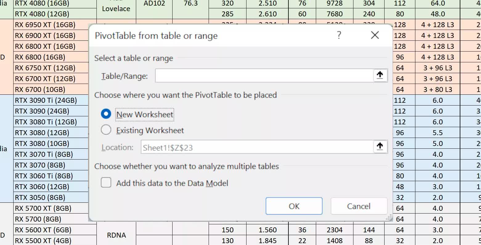
Let's say you have something like the table below and you just want to compare just a few parts of it – the first step is to press ALT, then N, V, and finally T.
A new window will pop open, make sure you select the entire table, including all column and row headers. Then decide if you want the pivot table to be in the same worksheet or a new one, and press enter.
You'll be faced with a blank table, and on the right side of the screen, a menu where you can select which columns you want to look at.
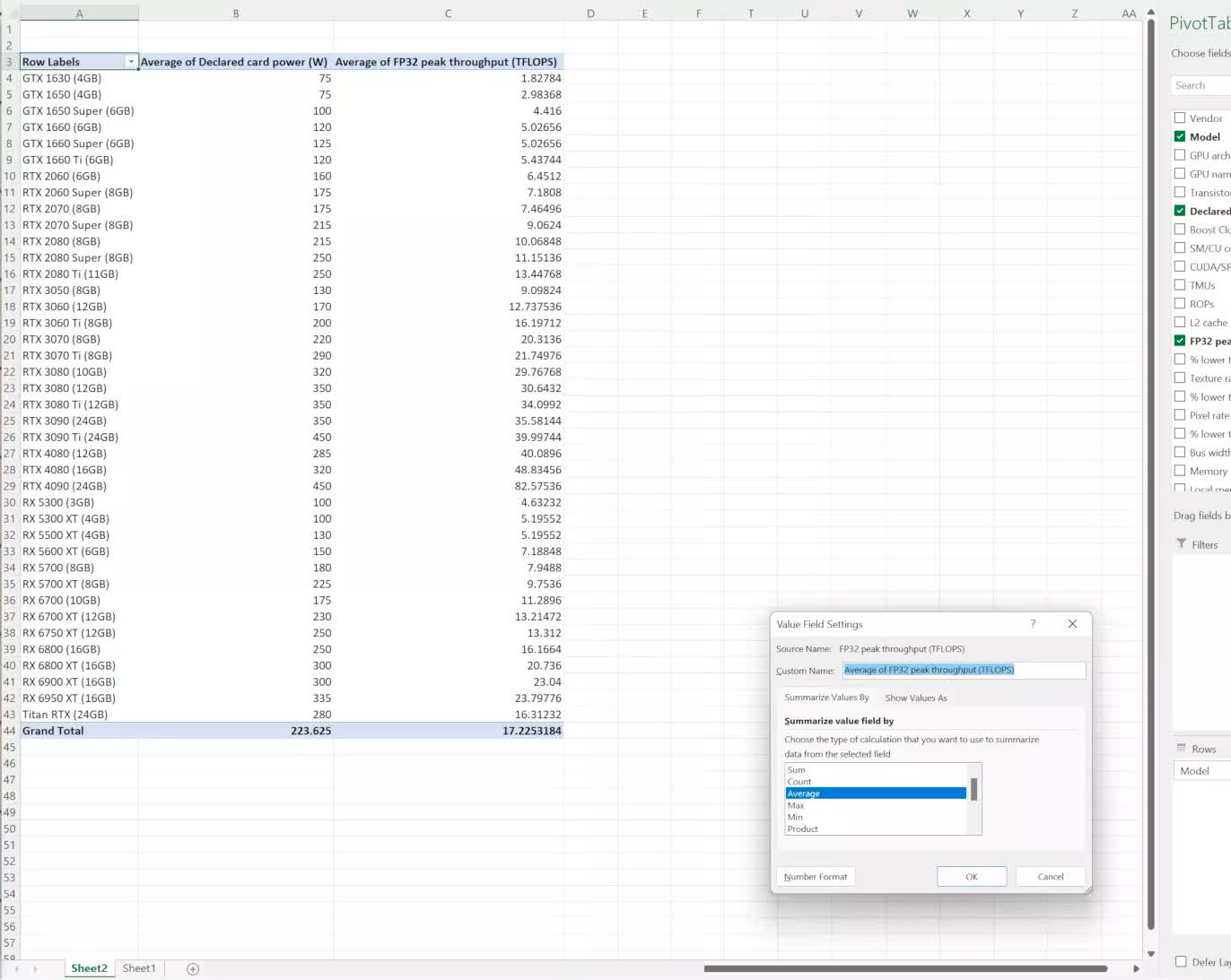
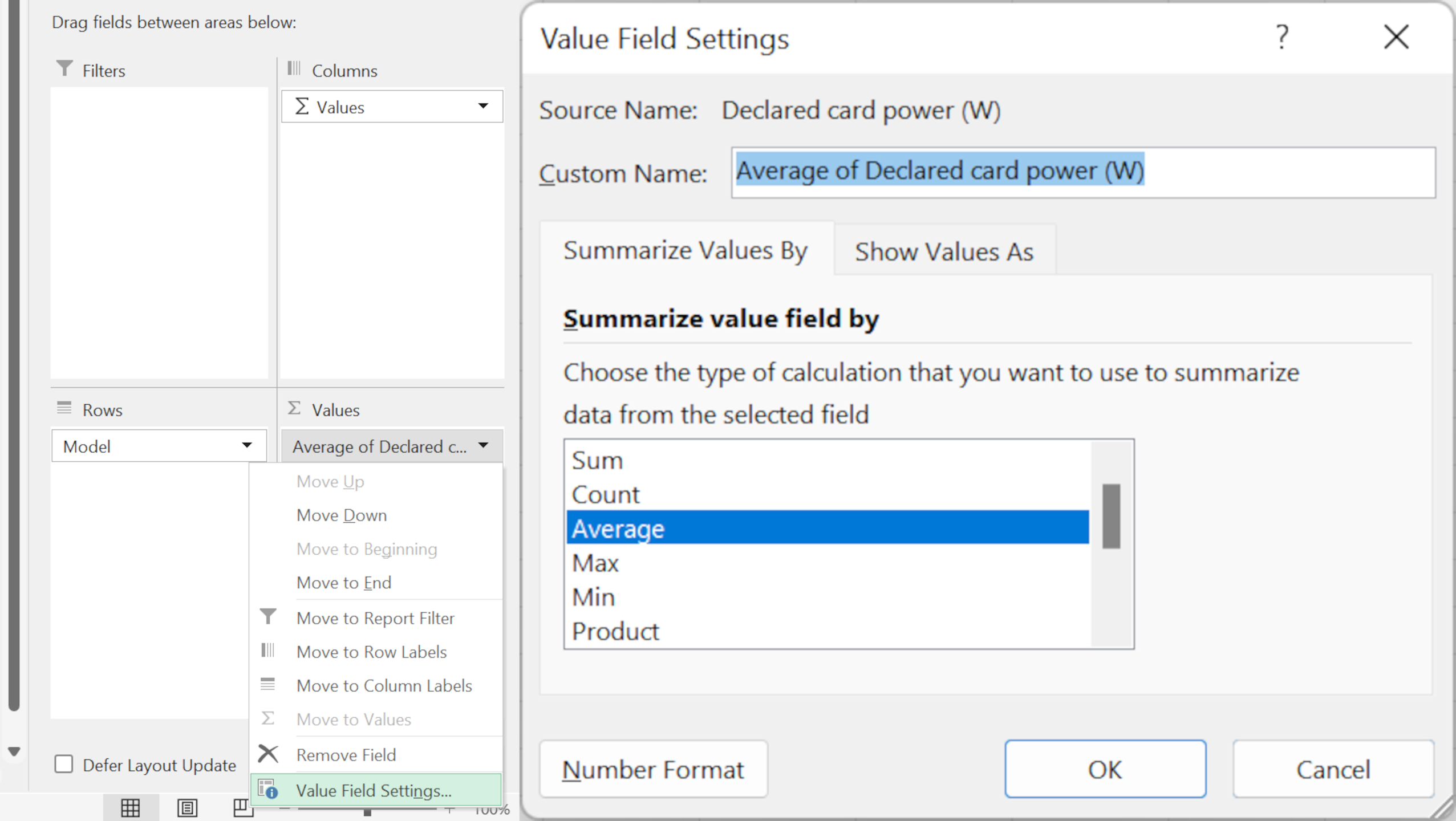
By default, the process adds a sum total to each column displayed, but that's easily changed by going to the Values section in the corner. Click on the drop-down menu arrow, select the bottom option, and hey presto!
Now you can add in your own custom label and change what's shown to a whole host of different summaries. Highlighting a summary cell, then pressing ALT, J, T, and then G will bring the options window back up again if you need to alter it.
Mastering the use of pivot tables can help productivity, or at the least, turn a big mess of data into something far more digestible.
8. Name your tables for nifty navigation
While it's perfectly possible to find values in a large table simply by using the Search function (CTRL+F), it's sometimes better to organize the whole thing by giving the various sections of the table a unique name.
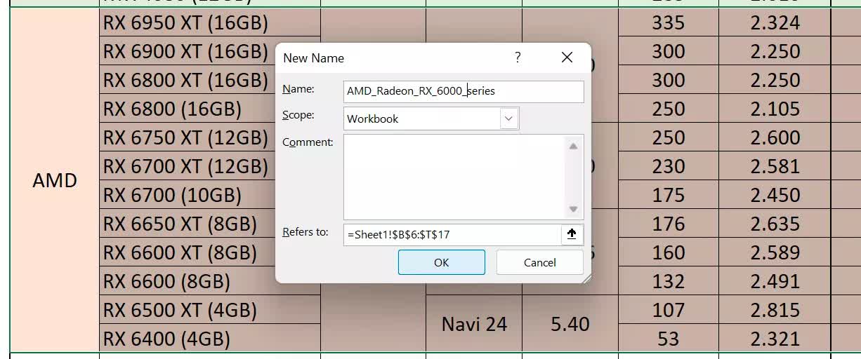
To do this, highlight the part of the table you want to name, then go to the Formulas section of the ribbon (ALT, M) or right-click on the highlighted section. You'll see the option to Define Name and clicking this will open up a new window.
Enter the name you want this section of the table to have; make sure you don't use any spaces. You can add comments at this stage to help others know what the name is referring to.
Once you've named all the parts you want, you can then navigate to them by using the Name Box, left of the formula field, or going to "View" on the Ribbon (ALT, W) and selecting Navigation (ALT, W, K).
Here you will see all of the named sections of the spreadsheet and click on any of these will jump you straight to that part. You can quickly edit or remove names by the Name Manager (ALT, M, N).
9. Flip data between rows and columns the pro way
If you have a table where the data is arranged in rows (horizontally) but you want it in columns, or the other way around, there's a quick way to do this. Highlight everything you want to change and then copy it (CTRL+C).
Then select a cell somewhere in the spreadsheet, right-click and select Paste Special. If the menu is a list of words, click on Transpose, but if you can only see a grid of icons, pick the one shown below.
This method works for changing from rows to columns and vice versa – you can even put the altered data over the original layout.
10. Fast facts about your data
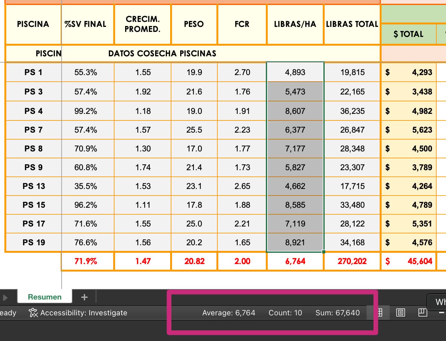
Sometimes, when looking at a big pile of values in a spreadsheet, all you want is a quick average, total, or even sum of a selection, rather than from an entire row or column. You can, of course, do this with a formula, but most recent versions of Excel do this automatically for any selection.
Highlight the values you want to examine and then look at the bottom bar of the Excel window...
You'll see average (arithmetic mean), count (number of cells), and the sum of the values. Click on any of them and that figure will be copied to the clipboard for later use.
So there you have it: 10 top tricks and hacks for Microsoft Excel. If you've got a great way of doing things with spreadsheets, share your knowledge in the comments section below.
You may also want to check out our Top 10 Hacks for Microsoft Word and Top 10 Hacks for PowerPoint.
